What is the effect of income on SGIP applications?
Introduction
Energy storage is poised for rapid growth and will play a major role in the decarbonization of our energy industry. 1 The California Public Utilities Commission (CPUC) created the Self Generation Incentive Program (SGIP), in part, to provide rebates to people and organizations looking to install energy storage systems. In September of 2019, they introduced additional funding for the “Equity” budget and a new funding category, “Equity Resiliency”. These funding categories aim to help lower-income, medically vulnerable, and at risk for fire communities pay for a battery. 2 Given that lower socioeconomic communities are shown to experience more frequent Public Safety Power Shutoffs (PSPS), 3 an energy storage system could be critical to avoiding the adverse effects of a power outage (e.g. food insecurity). There has been a study showing the socioeconomic disparities in residential battery storage adoption, 4 but there hasn’t been targeted analysis on SGIP participation post equity and equity resiliency funding becoming available.
Examining if there is an effect of income on SGIP applications for 2020, could help inform the effectiveness of the new funding categories and subsequent policy decisions.
Data
SGIP Applications
I downloaded SGIP application data from the California Distributed Energy Statistics site. 5 Application data is reported on a weekly basis via an excel file. For this analysis, SGIP applications were filtered down to just residential and single family battery applications for 2020. The data was then summarized by zip code to get total count of applications for each zip code. I did notice that the metadata didn’t always correctly specify the categorical values in each variable, so there is room for error in categorization.
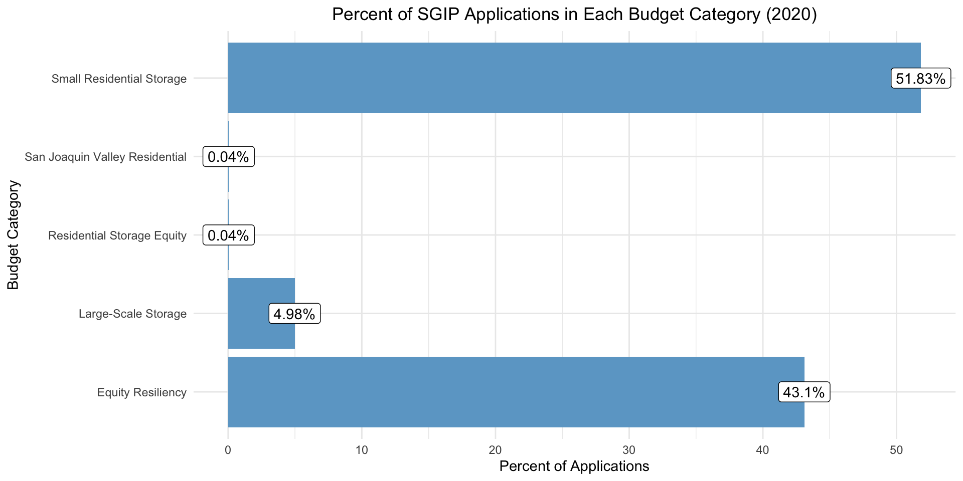
When visualizing SGIP applications for 2020, 43.14% of applications fall under the Equity and Equity Resiliency categories.
checkout the code
#loading the necessary pacakgeslibrary(tidyverse)library(readr)library(gt)library(tidycensus)library(janitor)library(lubridate)library(modelr)library(gridExtra)library(car)#setting file path for root directoryrootdir <- ("/Users/michelle/Documents/UCSB Grad School/Courses/eds_222/eds222_final_project")datadir <-(file.path(rootdir,"data"))#store and set API key to access tidycensuscensus_token <-Sys.getenv('CENSUS_KEY')census_api_key(census_token)#read in the SGIP datasgip <-read_csv(file.path(datadir,"sgip_weekly_data.csv")) |> janitor::clean_names()#filter down to rebates for just residential electrochemcial storage that were not cancelled, format date and zipsgip_res_battery <- sgip |>filter(equipment_type =="Electrochemical Storage", host_customer_sector %in%c("Residential", "Single Family"), budget_classification !="Cancelled") |>select("city", "county", "zip", "date_received", "budget_category", "host_customer_sector") |>mutate("date_received"=str_sub(date_received, 1, 8)) |>mutate("date_received"=as.Date(date_received, format ="%m/%d/%y")) |>mutate("year_received"=year(date_received)) |>mutate("month_received"=month(date_received)) |>mutate("zip"=ifelse(str_length(zip) ==10, substring(zip, 1, nchar(zip)-5), zip))#create sgip dataset filtered for 2020sgip_2020 <- sgip_res_battery |>filter(year_received ==2020)# create dataframe showing count of applications in each zip code for 2020sgip_zip_2020 <- sgip_2020 |>group_by(zip) |>summarize(count =n())#create a summary data frame showing applications by budget categorysgip_2020_budget <- sgip_2020 |>group_by(budget_category) |>summarize(count =n()) |>mutate(percent =round(((count/sum(count))*100),2), percent_label =paste0(percent, "%"))#plot percent SGIP applications by categoryggplot(sgip_2020_budget, aes(y = budget_category, x = percent)) +geom_bar(stat ="identity", fill ="skyblue3") +labs(title ="Percent of SGIP Applications in Each Budget Category (2020)", y ="Budget Category", x ="Percent of Applications") +theme_minimal() +theme(plot.title =element_text(hjust =0.5)) +geom_label(label = sgip_2020_budget$percent_label)
American Community Survey (ACS)
I accessed American Community Survey (ACS) data containing per capita income and population for each census tract in California through an API and the tidycensus package in R.6 ACS data is provided in tabular format and is read in as a data frame. ACS utilizes a stratified sampling approach, using address blocks to create strata.7 This could run the risk of the sample not reflecting the population if strata have overlapping characteristics. Additionally, data might not be as available/reliable for rural areas.8
checkout the code
#access ACS data variables for 2020 year v20 <-load_variables(2020, "acs5", cache =TRUE)#read in per capita income data for census tracts in CAca_pc_income_tract <-get_acs(geography ="tract",variables =c(percapita_income ="B19301_001"),state ="CA",year =2020)#clean and format per capita income data frameca_pc_income_tract_clean <- ca_pc_income_tract |>select(c("GEOID", "NAME", "estimate")) |>rename(percapita_income ="estimate")#read in population data for census tracts in CAca_pop_tract <-get_acs(geography ="tract",variables =c(population ="B01003_001"),state ="CA",year =2020)#clean and format population data frame ca_pop_tract_clean <- ca_pop_tract |>select(c("GEOID", "NAME", "estimate")) |>rename(population ="estimate")#combine per capita income and population data framescombine_census <-cbind(ca_pc_income_tract_clean, ca_pop_tract_clean$population) |>rename(population ="ca_pop_tract_clean$population", tract ="GEOID")
U.S. Department of Housing and Urban Development (HUD)
I downloaded the crosswalk file in the form of a csv from the U.S. HUD site. 9 The file relates zip codes to census tracts and was utilized to match up application data (zip code level) to per capita income and population data (census tract level).
checkout the code
#read in crosswalk file to use when matching zip codes to census tractscrosswalk <-read_csv(file.path(datadir,"ZIP_TRACT_122020.csv")) |> janitor::clean_names()
Analysis
To analyze the effect of income on SGIP applications, I utilized the three datasets outlined above to create a data frame showing applications per thousand people and per capita income for each zip code. When aggregating from census tract level to zip code level, I took the median per capita income and summed the populations in each census tract to get income and population variables for each zip code. I used population of each zip code to calculate the applications per thousand people in order to account for the fact that higher income areas have more people and to create a more appropriate scale for interpretation. I did notice that after combining the datasets, there were 1,933 NA values for per capita income and 1,896 NA values for population out of the 10,978 census tracts in the dataset. This could lead to inaccuracies since observations are analyzed on the zip code level and aggregation of the census tract data was performed.
checkout the code
#combine sgip_zip_2020 and crosswalk file by zip to get a data frame with sgip applications per census tract#because there are multiple census tracts for one zip code, use the res_ratio to allocate what portion of the count of SGIP applications should be allocated to one census tractsgip_zip_census <-left_join(sgip_zip_2020, crosswalk, by ="zip") |>mutate("count_adjusted"= count*res_ratio) #now we have theoretical count of applications per census tract#combine sgip_zip_census with acs data by tractcombined_all <-left_join(sgip_zip_census, combine_census, by ="tract") |>mutate("percapita_application"= count_adjusted/population) |>mutate("applications_per_thousand"= (count_adjusted/population)*1000) |>select(c(-"oth_ratio", -"tot_ratio", -"bus_ratio"))#take the combined_all data frame and consolidate back to apps per zip (averaging per capita income and summing population of each census tract into zip codes)combined_by_zip <- combined_all |>group_by(zip) |>summarize(applications =mean(count, na.rm =TRUE), percapita_income =median(percapita_income, na.rm =TRUE), population =sum(population, na.rm =TRUE)) |>filter(!is.na(percapita_income)) |>mutate("applications_per_1000_people"= (applications/population)*1000, "percapita_application"= applications/population)
Regression Models
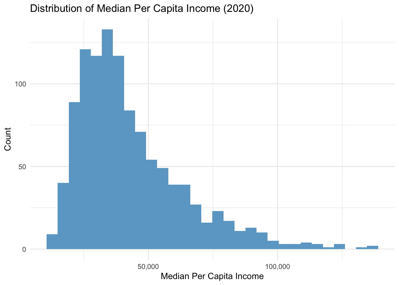
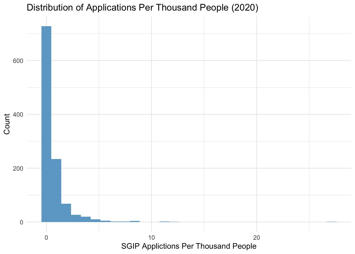
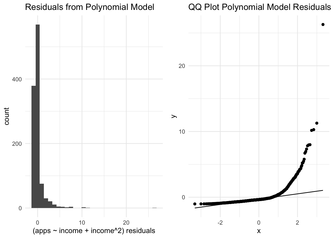
Next, I ran different regression models to see what would best fit the data. I started with a simple linear regression, but noticed that the median per capita income and the applications per thousand people observations were not normally distributed with a right tail (see supporting figures). Therefore, I ran a linear-log regression and log-log regression. The residuals from these models were not normally distributed so I ran a polynomial regression. The residuals on the polynomial regression were not normal either (see supporting figures), but I concluded that the polynomial regression was best fit since visually the slope doesn’t look constant and the coefficients were significant. Here is the equation for the model: \[application_i =\beta_{0}+\beta_{1} \cdot income_i + \beta_{2} \cdot income_i^2 + \varepsilon_i\]
I did notice that there was an outlier in the dataset, but when I removed the outlier and ran the polynomial regression it did not change the significance of the coefficients. Because the outlier didn’t drastically change model results and there was no evidence that this data point was an outlier caused by data entry or measurement errors, I left it in.
As mentioned above, on all the models tested the residuals were not normally distributed with a long right tail. This means that the amount of error in the model is not consistent across the full range of my observed data and the model’s ability to accurately predict applications per thousand people at a given median per capita income could be low.
Hypothesis Testing
I jointly tested the \(\beta_{1}\) and \(\beta_{2}\) coefficients using the linearHypothesis() function from the car package to test for no relationship between median per capita income and applications per thousand people.
\(H_0: \beta_{1} = 0, \beta_{2} = 0\)
\(H_A: \beta_{j}\neq 0\) for at least one \(j = 1,2\)
Results
Polynomial Regression
From the below outputs of the model, I can see that the coefficient of per capita income is statistically significant at the 0.1% significance level (p-value = 0.0003) and the coefficient of per capita income squared is statistically significant at the 1% significance level (p-value = 0.0088). The R squared and adjusted R squared are really low at 0.022 and 0.02, respectively. This means that 2% of the variability in applications per thousand people is explained by median per capita income. Having a low R squared value and a high significance for the coefficients in the model could mean that there is a statistically significant relationship between applications and income, but the predictive accuracy of the model is low.
checkout the code
#polynomial regressionpoly_model <-lm(applications_per_1000_people ~ percapita_income +I(percapita_income^2), data = combined_by_zip)#store all the values of the model R2_poly_model =summary(poly_model)$r.squaredR2_poly_adjusted =summary(poly_model)$adj.r.squaredintercept_poly <-summary(poly_model)$coefficients["(Intercept)", "Estimate"]b1_poly <-summary(poly_model)$coefficients["percapita_income", "Estimate"]b2_poly <-summary(poly_model)$coefficients["I(percapita_income^2)", "Estimate"]Predictors <-c("Intercept", "per capita income", "(per capita income)^2")Estimate <-signif(summary(poly_model)$coefficients[,"Estimate"], digits =3)SE <-signif(summary(poly_model)$coefficients[,"Std. Error"], digits =3)p <-round(summary(poly_model)$coefficients[,"Pr(>|t|)"], 4)poly_model_summary <-data.frame(Predictors, Estimate, SE, p)#create table of regression outputgt_summary <- poly_model_summary |>gt() |>tab_header(title ="Polynomial Model Output Summary" ) |>tab_footnote(footnote ="Observations: 1104") |>tab_footnote(footnote =paste("R^2/R^2 adjusted:", round(R2_poly_model,3), "/", round(R2_poly_adjusted,3)) )gt_summary
Polynomial Model Output Summary
Predictors
Estimate
SE
p
Intercept
-1.69e-01
2.08e-01
0.4186
per capita income
2.95e-05
8.12e-06
0.0003
(per capita income)^2
-1.80e-10
6.85e-11
0.0088
Observations: 1104
R^2/R^2 adjusted: 0.022 / 0.02
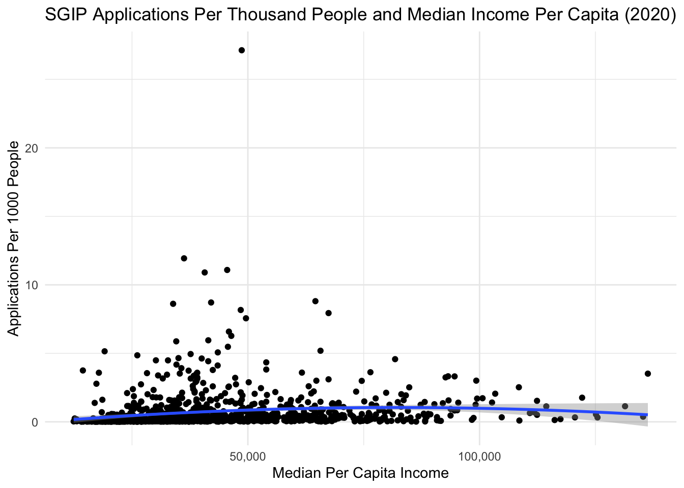
When looking at the below graph and resulting formula, we can conclude that the effect of an increase on median per capita income on applications per thousand people depends on the baseline level of median per capita income.
checkout the code
#plotggplot(data = combined_by_zip, aes(x = percapita_income, y = applications_per_1000_people)) +geom_point() +geom_smooth(method ="lm", formula = y ~ x +I(x^2), size =1) +scale_x_continuous(name="Median Per Capita Income", labels = scales::comma) +labs(x ="Median Per Capita Income", y ="Applications Per 1000 People", title ="SGIP Applications Per Thousand People and Median Income Per Capita (2020)") +theme_minimal()
To interpret output from the model, we can look at the difference in predicted applications per thousand people between regions of median per capita income.
When moving from a median per capita income of $15,000 to $25,000 (low income), predicted applications per thousand people increases by 0.22. When moving from a median per capita income of $60,000 to $70,000 (middle income), predicted applications per thousand people increases by 0.06. When moving from a median per capita income of $100,000 to $110,000 (high income), predicted applications per thousand people decreases by 0.08.
checkout the code
#create a function out of the polynomial regressionapp_pred_function <-function(income){return(intercept_poly + (b1_poly * income) + (b2_poly * (income^2)))}#predicted applications per 1000 people for per capita income of 15,000 vs. 25,000pred_15000 <-app_pred_function(income =15000)pred_25000 <-app_pred_function(income =25000)diff_pred_low <- pred_25000 - pred_15000diff_pred_low#predicted applications per 1000 people for per capita income of 60,000 vs. 70,000pred_60000 <-app_pred_function(income =60000)pred_70000 <-app_pred_function(income =70000)diff_pred_mid<- pred_70000 - pred_60000diff_pred_mid#predicted applications per 1000 people for per capita income of 100,000 vs. 110,000pred_100000 <-app_pred_function(income =100000)pred_110000 <-app_pred_function(income =110000)diff_pred_high <- pred_110000- pred_100000diff_pred_high
Hypothesis Testing
The resulting F-statistic (12.39) and p-value (4.76e-06) from the hypothesis testing indicate that I can reject my null hypothesis that both coefficients are 0 (i.e. there is no relationship between median per capita income and applications per thousand people).
checkout the code
#jointly test if beta1 and beta 2 are 0, test that there is no relationship at all between y and xlinearHypothesis(poly_model,c("percapita_income = 0", "I(percapita_income^2) = 0"))
Conclusion and Next Steps
From the results of this analysis, I can conclude that income does have an effect on SGIP applications. It is hard to definitely say that the SGIP program is or is not helping lower income communities since the slope of the model increases up until a certain point and then decreases. From previous research mentioned in the introduction, I would have thought the slope of the model would be consistently positive. This would have shown that the SGIP program was being utilized less by low income communities. The model does, however, conclude that the lowest income communities are not utilizing the SGIP program. This can be due to a number of factors including, but not limited to, energy storage systems often being paired with solar, requirements of home ownership, and a lengthy rebate process that are barriers to adoption of this program. Some further analysis that would help determine if the equity and equity resiliency funding is helping low income communities is to compare pre 2020 applications to post 2020 applications to get a sense of the change in program participation among low income communities. Also adding medical vulnerability and wildfire risk as predictors to the model could indicate if those communities are utilizing the program and control for interactions between income and these additional variables.
#histogram for per capita incomeggplot(data = combined_by_zip) +geom_histogram(aes(percapita_income), fill ="skyblue3") +scale_x_continuous(name="Median Per Capita Income", labels = scales::comma) +labs(title ="Distribution of Median Per Capita Income (2020)", y ="Count") +theme_minimal()
checkout the code
#histogram for applications per 1000 peopleggplot(data = combined_by_zip) +geom_histogram(aes(applications_per_1000_people), fill ="skyblue3") +labs(x ="SGIP Applictions Per Thousand People", y ="Count", title ="Distribution of Applications Per Thousand People (2020)") +theme_minimal()
checkout the code
#get a predicted value for every observation (generate a column of predictions called pred)#then use predictions to compute residuals (actual - prediction) -> add column called residualspredictions_4 <- combined_by_zip |>add_predictions(poly_model) |>mutate(residuals = applications_per_1000_people - pred)#test assumption that errors are normally distributedpoly_residuals_hist <-ggplot(data = predictions_4) +geom_histogram(aes(residuals)) +labs(title ="Residuals from Polynomial Model", x ="(apps ~ income + income^2) residuals") +theme_minimal()poly_income_qq <-ggplot(data = predictions_4,aes(sample = residuals)) +geom_qq() +geom_qq_line() +labs(title ="QQ Plot Polynomial Model Residuals") +theme_minimal()grid.arrange(poly_residuals_hist, poly_income_qq, ncol =2)
References
Footnotes
Blair, Nate, Chad Augustine, Wesley Cole, et al. 2022. Storage Futures Study: Key Learnings for the Coming Decades. Golden, CO: National Renewable Energy Laboratory. NREL/TP-7A40-81779. https://www.nrel.gov/docs/fy22osti/81779.pdf↩︎
Auth, CPUC. “Participating in Self-Generation Incentive Program (SGIP).” California Public Utilities Commission, 2020, https://www.cpuc.ca.gov/industries-and-topics/electrical-energy/demand-side-management/self-generation-incentive-program/participating-in-self-generation-incentive-program-sgip.↩︎
Vilgalys, Max. “Equity and Adaptation to Wildfire Risk: Evidence from California Public Safety Power Shutoffs.” (2022).↩︎
David P. Brown, Socioeconomic and demographic disparities in residential battery storage adoption: Evidence from California, Energy Policy, Volume 164, 2022, 112877, ISSN 0301-4215, https://doi.org/10.1016/j.enpol.2022.112877. (https://www.sciencedirect.com/science/article/pii/S0301421522001021)↩︎
Bureau, US Census. “Design and Methodology Report.” Census.gov, 14 Dec. 2021, https://www.census.gov/programs-surveys/acs/methodology/design-and-methodology.html.↩︎
Research and Training Center on Disability in Rural Communities. (2017). Data limitations in the American Community Survey (ACS): The impact on rural disability research. Missoula, MT: The University of Montana Rural Institute for Inclusive Communities.↩︎